Optimization Methods of GerryChain
In GerryChain, we provide a class known as the SingleMetricOptimizer as well as a
Gingelator subclass that allow us to perform optimization runs.
Currently, there are 3 different optimization methods available in GerryChain:
Short Bursts: This method chains together a series of neutral explorers. The main idea is to run the chain for a short period of time (short burst) and then continue the chain from the partition that maximizes the objective function within the most recent short burst. For more information, please refer to this paper.
Simulated Annealing: This method varies the probablity of accepting a worse plan according to a temperature schedule which ranges from 0 to 1.
Tilted Runs: This method accepts a worse plan with a fixed probability \(p\), and always accepts better plans.
While sampling naively with GerryChain can give us an understanding of the neutral baseline for a state, there are often cases where we want to find plans with properties that are rare to encounter in a neutral run. Many states have laws/guidelines that state that plans should be as compact as feasibly possible, maximize preservation of political boundaries and/or communities of interest; some even look to minimize double bunking of incumbents or seek proportionality/competitiveness in contests. Heuristic optimization methods can be used to find example plans with these properties and to explore the trade-offs between them.
For the first part of this documentation, we will be working with a simple example wherein
we will try to minimize the number of cut edges in a partition. There are, of course
more complex things that we can do here, but the point of this guide is to just get you
used to the API for the SingleMetricOptimizer class. As per usual, we will begin
with importing the necessary packages:
from gerrychain import (GeographicPartition, Partition, Graph, MarkovChain,
                        proposals, updaters, constraints, accept, Election)
from gerrychain.optimization import SingleMetricOptimizer, Gingleator
from gerrychain.tree import recursive_seed_part
from functools import partial
import pandas as pd
import json
from networkx.readwrite import json_graph
import matplotlib.pyplot as plt
from tqdm import tqdm
import numpy as np
import random

random.seed(2024)
Since the SingleMetricOptimizer class uses ReCom under the hood, we will need to
do a lot of the same setup that we did in the Running a Chain with ReCom
section:
graph = Graph.from_json("05_bg_census_consolidated.json")

POPCOL = "tot_pop_20"
SEN_DISTS = 35
EPS = 0.02
TOTPOP = sum(graph.nodes()[n][POPCOL] for n in graph.nodes())

chain_updaters = {
    "population": updaters.Tally(POPCOL, alias="population"),
}

initial_partition = Partition.from_random_assignment(
    graph=graph,
    n_parts=SEN_DISTS,
    epsilon=EPS,
    pop_col=POPCOL,
    updaters=chain_updaters
)

proposal = partial(
    proposals.recom,
    pop_col=POPCOL,
    pop_target=TOTPOP/SEN_DISTS,
    epsilon=EPS,
    node_repeats=1
)

chain_constraints = constraints.within_percent_of_ideal_population(initial_partition, EPS)
Using SingleMetricOptimizer
SingleMetricOptimizer is a wrapper around our basic MarkovChain
class; to set it up, we simply pass it a proposal function, some constraints, an initial
state, and the objective function of interest:
def num_cut_edges(partition):
    return len(partition["cut_edges"])

optimizer = SingleMetricOptimizer(
    proposal=proposal,
    constraints=chain_constraints,
    initial_state=initial_partition,
    optimization_metric=num_cut_edges,
    maximize=False
)
An important thing to note here is that the objective function that we are passing takes as
input a Partition object and returns a float or integer value. In our case, one of the
default updaters for the Partition class, cut_edges, returns the cut edge set for
the whole partition. With this, we can run each of the optimization methods and collect some data!
Note
We collect data using the syntax optimizer.best_score. The .best_score property
of the SingleMetricOptimizer just returns the best score that has been observed
throughout the duration of the optimization process. To evaluate the score of a
particular partition, we can use the syntax optimizer.score(partition).
total_steps = 10000

# Short Bursts
min_scores_sb = np.zeros(total_steps)
scores_sb = np.zeros(total_steps)
for i, part in enumerate(optimizer.short_bursts(5, 2000, with_progress_bar=True)):
    min_scores_sb[i] = optimizer.best_score
    scores_sb[i] = optimizer.score(part)

# Simulated Annealing
min_scores_anneal = np.zeros(total_steps)
scores_anneal = np.zeros(total_steps)
for i, part in enumerate(
    optimizer.simulated_annealing(
        total_steps,
        optimizer.jumpcycle_beta_function(200, 800),
        beta_magnitude=1,
        with_progress_bar=True
    )
):
    min_scores_anneal[i] = optimizer.best_score
    scores_anneal[i] = optimizer.score(part)

# Tilted Runs
min_scores_tilt = np.zeros(total_steps)
scores_tilt = np.zeros(total_steps)
for i, part in enumerate(optimizer.tilted_run(total_steps, p=0.125, with_progress_bar=True)):
    min_scores_tilt[i] = optimizer.best_score
    scores_tilt[i] = optimizer.score(part)
We can then plot the results to see how each method performed:
fig, ax = plt.subplots(figsize=(12,6))
plt.plot(min_scores_sb, label="Short Bursts")
plt.plot(min_scores_anneal, label="Simulated Annealing")
plt.plot(min_scores_tilt, label="Tilted Run")
plt.xlabel("Steps", fontsize=20)
plt.ylabel("Min #CutEdges Observered", fontsize=20)
plt.legend()
plt.show()
This should give you something like:
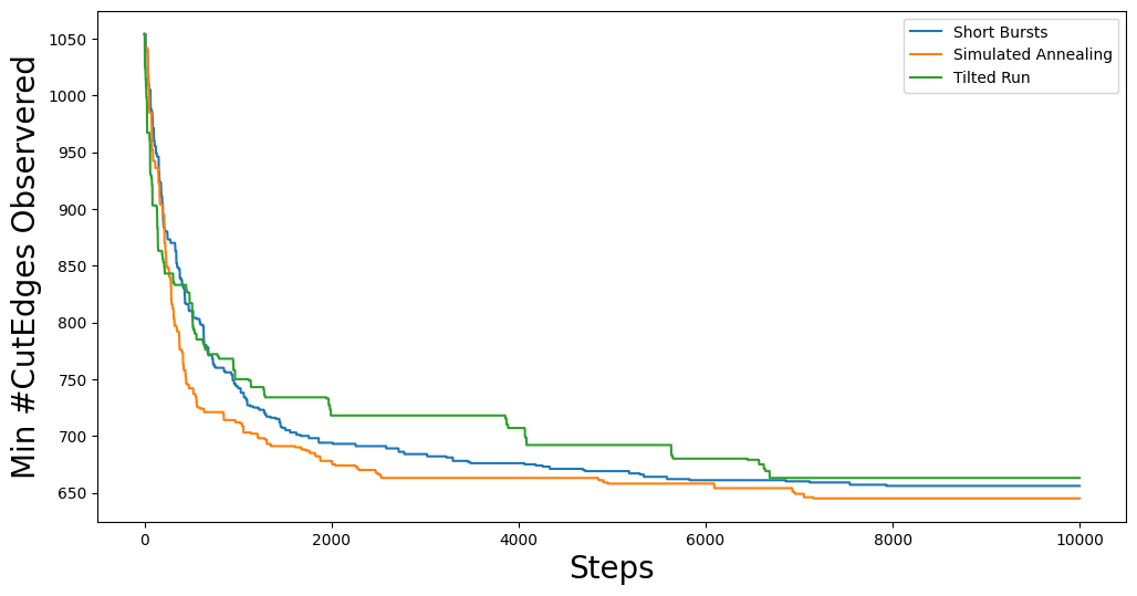
Of course, the above trace is just shows the progression of the best score as the chain moves along. If we want to see how the optimization function performs at each step, we can plot the full trace:
fig, ax = plt.subplots(figsize=(12,6))
plt.plot(scores_sb, label="Short Bursts")
plt.plot(scores_anneal, label="Simulated Annealing")
plt.plot(scores_tilt, label="Tilted Run")
plt.xlabel("Steps", fontsize=20)
plt.ylabel("Cut Edges", fontsize=20)
plt.legend(fontsize=9)
plt.show()
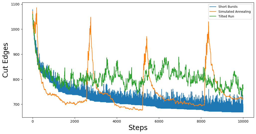
Here we can see some of the quirks of each of the optimization methods. For example, our simulated annealing method is using a jumpcycle beta function and we can see when the acceptance rate is high represented by spikes in the trace plot. Short bursts is generally pretty noisy, but since each burst starts from the best partition in the previous burst, we see that it has a general downward trend. Lastly, tilted runs just accept worse partitions with a fixed probability, so the (relatively) uniform volatility of the cut edge score trace plot is expected.
Using Gingleator
Named for the Supreme Court case Thornburg v. Gingles, Gingles’ Districts are districts that are 50% + 1 of a minority population subgroup (more colloquially called majority-minority districts).
Gingleator is a subclass of the SingleMetricOptimizer. Technically this means that
everything in the Gingleator class can also be done using the SingleMetricOptimizer
class, but the Gingleator class provides some quality-of-life improvements to the user
experience.
For the purposes of this tutorial, we will be using the Gingleator class to try and optimize
the number of districts with
A majority-minority population for black population (mainly as a warm-up)
A majority-minority Voting Age Population (VAP) for black voters
In the provided JSON file (linked in the blue button above), we have included the following columns aggregated from the 2020 Census data on block groups for the state of Arkansas:
tot_pop_20: Total Population for the block group according to the 2020 Censustot_vap_20: Total Voting Age Population (18+) for the block group according to the 2020 Censusbpop_20: Total Black Population for the block group according to the 2020 Censusbvap_20: Total Black Voting Age Population (18+) for the block group according to the 2020 Census
Note
Both the bpop_20 and bvap_20 columns are “any part black” aggregations acquired
from the 2020 Census P1 and P3 tables. That is to say, bpop_20 is the total number of people
that included “black” as any part of their racial identity when reporting to the Census Bureau.
Since the Gingleator class is a subclass of SingleMetricOptimizer, a lot of the
setup for the optimization process is the same. The main things that we need to be careful of
are the parameters we pass to the Gingleator class. Specifically, we need to make updaters
that keep track of the relevant statistics we are optimizing for. In example (1) this means
that we need an updater for the total population (we will just call this population) and
the total black population (we will call this bpop).
Majority-Minority Total Population
graph = Graph.from_json("05_bg_census_consolidated.json")

POPCOL = "tot_pop_20"
SEN_DISTS = 35
EPS = 0.02
TOTPOP = sum(graph.nodes()[n][POPCOL] for n in graph.nodes())

# ========================================================
# WE HAVE UPDATED SOME THINGS IN HERE! MAKE SURE TO CHECK!
# ========================================================
chain_updaters = {
    "population": updaters.Tally(POPCOL, alias="population"),
    "bpop": updaters.Tally("bpop_20", alias="bpop"),
}

initial_partition = Partition.from_random_assignment(
    graph=graph,
    n_parts=SEN_DISTS,
    epsilon=EPS,
    pop_col=POPCOL,
    updaters=chain_updaters
)

proposal = partial(
    proposals.recom,
    pop_col=POPCOL,
    pop_target=TOTPOP/SEN_DISTS,
    epsilon=EPS,
    node_repeats=1
)

chain_constraints = constraints.within_percent_of_ideal_population(initial_partition, EPS)
There are several parameters that we need to pass to the Gingleator class. Most of them
should be familiar at this point, but the following are the most important ones for
understanding appropriate usage of the class:
Population Parameters of the Gingleator class
There are three main population parameters that we can to pass to the Gingleator class.
However, depending on which are passed, either one or two of them will be unnecessary.
(
minority_pop_col,total_pop_col): This pair is passed when the user would like for theGingleatorclass to compute the percentage of the minority population from quotient of these two updaters. Thetotal_pop_colis the name of the UPDATER that contains the total population for each partition, and theminority_pop_colis the name of the UPDATER that contains total population for the minority population of interest. In the case that this pair of parameters is passed, the initialization function will create an updater forminority_perc_colvia the formulaminority_pop_col / total_pop_colfor each partition, and the optimization function will then be passed the decimal values to compute the resulting partition’s score for each step in the Markov chain.The
minority_perc_colis the name of the UPDATER that contains the percentage of the minority population of interest. The updater should already have the score for each part in the partition formatted as a percentage, so the optimization function will process these values as they are passed.
Score Function of the Gingleator class
The score_function parameter is a function \(f:P \to \mathbb{R}\) that
take in a gerrychain Partition object and returns a score for that partition. The
SingleMetricOptimizer class also allows for the modification of score functions, but
the Gingleator class comes with some nice built-in score functions that are meant to
to be used as good starting points for exploring the space of possible plans.
Let \(t\) be the threshold for the score as determined by the user, and let \(n\) be the number of districts in a partition \(P\) with a minority percentage over the threshold value \(t\), so \(n = \sum_{p_i \in P} \mathbb{1}_{p_i\geq t}\) where \(p_i\) is the percentage of the minority population in district \(i\).
num_opportunity_dists: Given aPartition, this function will return \(n\).reward_partial_dist: Given aPartition, this function will return \(n + \max(\{p_i : p_i < t\})\).reward_next_highest_close: Given aPartition, let \(p_k = \max(\{p_i : p_i < t\})\). This function will return \(n\) if \(p_k + 0.1 < t\) and \(n + 10(p_k - t + 0.1)\) otherwise.penalize_maximum_over: Given aPartition, this function will return 0 if \(n = 0\) and \(n - \frac{1-\max(\{p_i\})}{1-t}\) otherwise.penalize_avg_over: Given aPartition, this function will return 0 if \(n = 0\) and \(n - \frac{1-avg(\{p_i: p_i \geq t\})}{1-t}\) otherwise.
We are now prepared to instantiate the Gingleator class:
gingles = Gingleator(
    proposal,
    chain_constraints,
    initial_partition,
    minority_pop_col='bpop',
    total_pop_col='population',
    score_function=Gingleator.reward_partial_dist
)
Since the Gingleator class is a subclass of the SingleMetricOptimizer class, we can
use the same optimization methods as before:
total_steps = 10000

# Short Bursts
max_scores_sb = np.zeros(total_steps)
scores_sb = np.zeros(total_steps)
for i, part in enumerate(gingles.short_bursts(10, 1000, with_progress_bar=True)):
    max_scores_sb[i] = gingles.best_score
    scores_sb[i] = gingles.score(part)

# Simulated Annealing
max_scores_anneal = np.zeros(total_steps)
scores_anneal = np.zeros(total_steps)
for i, part in enumerate(
    gingles.simulated_annealing(
        total_steps,
        gingles.jumpcycle_beta_function(1000, 4000),
        beta_magnitude=500,
        with_progress_bar=True
    )
):
    max_scores_anneal[i] = gingles.best_score
    scores_anneal[i] = gingles.score(part)

# Tilted Runs
max_scores_tilt = np.zeros(total_steps)
scores_tilt = np.zeros(total_steps)
for i, part in enumerate(gingles.tilted_run(total_steps, 0.125, with_progress_bar=True)):
    max_scores_tilt[i] = gingles.best_score
    scores_tilt[i] = gingles.score(part)
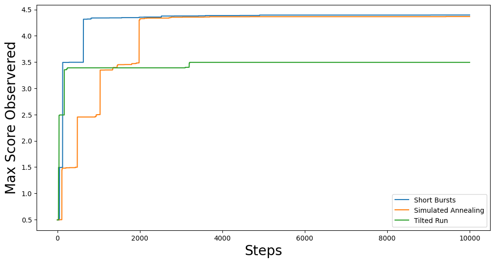
And we can plot the results again:
fig, ax = plt.subplots(figsize=(12,6))
plt.plot(max_scores_sb, label="Short Bursts")
plt.plot(max_scores_anneal, label="Simulated Annealing")
plt.plot(max_scores_tilt, label="Tilted Run")
plt.xlabel("Steps", fontsize=20)
plt.ylabel("Max Score Observered", fontsize=20)
plt.legend()
plt.show()
This should give you something like:
Great! We have successfully used the Gingleator class to optimize the number of districts
with a majority-minority population for black population. Now, we can do the same thing for
for the majority-minority Voting Age Population (VAP) for black voters.
Majority-Minority Voting Age Population
The astute reader will probably notice pretty quickly that there is a very easy way to modify the code from the previous section to optimize for Majority-Minority VAP. Indeed, all we need to do is change our updaters to be
chain_updaters = {
    "population": updaters.Tally(POPCOL, alias="population"),
    "vap": updaters.Tally("tot_vap_20", alias="vap"),
    "bvap": updaters.Tally("bvap_20", alias="bvap"),
}
and then change our Gingleator class instantiation to be
gingles = Gingleator(
    proposal,
    chain_constraints,
    initial_partition,
    minority_pop_col='bvap',
    total_pop_col='vap',
    score_function=Gingleator.reward_partial_dist
)
and we will be off to the races. In the interest of being thorough, however, let us see how to
modify this code to make use of the minority_perc_col parameter of the Gingleator class.
For this, we will just need to tweak our updaters a little bit:
graph = Graph.from_json("05_bg_census_consolidated.json")

POPCOL = "tot_pop_20"
SEN_DISTS = 35
EPS = 0.02
TOTPOP = sum(graph.nodes()[n][POPCOL] for n in graph.nodes())


# Updaters take in partitions and then return some value. In this case, we
# want to return a dictionary of mapping each part in the partition to the value BVAP/VAP
def compute_bvap_pct(partition):
    percent_by_part = {}
    for part in partition.parts:
        # bvap and vap are dictionaries mapping each partition part to
        # it corresponding BVAP or VAP tally respectively
        percent_by_part[part] = partition["bvap"][part] / partition["vap"][part]
    return percent_by_part

# ========================================================
# WE HAVE UPDATED SOME THINGS IN HERE! MAKE SURE TO CHECK!
# ========================================================
chain_updaters = {
    "population": updaters.Tally(POPCOL, alias="population"),
    "vap": updaters.Tally("tot_vap_20", alias="vap"),
    "bvap": updaters.Tally("bvap_20", alias="bvap"),
    "bvap_pct": compute_bvap_pct
}

initial_partition = Partition.from_random_assignment(
    graph=graph,
    n_parts=SEN_DISTS,
    epsilon=EPS,
    pop_col=POPCOL,
    updaters=chain_updaters
)

proposal = partial(
    proposals.recom,
    pop_col=POPCOL,
    pop_target=TOTPOP/SEN_DISTS,
    epsilon=EPS,
    node_repeats=1
)

chain_constraints = constraints.within_percent_of_ideal_population(initial_partition, EPS)
gingles = Gingleator(
    proposal,
    chain_constraints,
    initial_partition,
    minority_perc_col='bvap_pct',
    score_function=Gingleator.reward_partial_dist
)
total_steps = 10000

# Short Bursts
max_scores_sb = np.zeros(total_steps)
scores_sb = np.zeros(total_steps)
for i, part in enumerate(gingles.short_bursts(10, 1000, with_progress_bar=True)):
    max_scores_sb[i] = gingles.best_score
    scores_sb[i] = gingles.score(part)

# Simulated Annealing
max_scores_anneal = np.zeros(total_steps)
scores_anneal = np.zeros(total_steps)
for i, part in enumerate(
    gingles.simulated_annealing(
        total_steps,
        gingles.jumpcycle_beta_function(1000, 4000),
        beta_magnitude=500,
        with_progress_bar=True
    )
):
    max_scores_anneal[i] = gingles.best_score
    scores_anneal[i] = gingles.score(part)

# Tilted Runs
max_scores_tilt = np.zeros(total_steps)
scores_tilt = np.zeros(total_steps)
for i, part in enumerate(gingles.tilted_run(total_steps, 0.125, with_progress_bar=True)):
    max_scores_tilt[i] = gingles.best_score
    scores_tilt[i] = gingles.score(part)
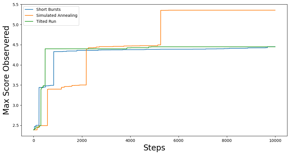
And now we plot the results again!
fig, ax = plt.subplots(figsize=(12,6))
plt.plot(max_scores_sb, label="Short Bursts")
plt.plot(max_scores_anneal, label="Simulated Annealing")
plt.plot(max_scores_tilt, label="Tilted Run")
plt.xlabel("Steps", fontsize=20)
plt.ylabel("Max Score Observered", fontsize=20)
plt.legend()
plt.show()