Using maup to import a real-life plan in GerryChain
To generate an ensemble of districting plans using GerryChain, we need a
starting point for our Markov chain. GerryChain gives you functions like
recursive_tree_part to generate such plans from scratch, but you may want to
use an actual districting plan from the real world instead. You also may want to
compare a real-life plan to your ensemble.
maup is MGGG’s package for doing common
spatial data operations with redistricting data. We’ll use this package to
assign our basic geographic units to the districts in the plan we’re interested
in. Our steps are:
Download a Shapefile of the districting plan we’re interested in,
Use
maupto assign the our basic units to the districts in that plan, and thenCreate a GerryChain Partition using that assignment.
>>> import maup
>>> import geopandas
>>> import matplotlib.pyplot as plt
Downloading a plan
For this guide, we’ll assign Massachusetts’s block groups to the 2010 Massachusetts State Senate districting plan. We can use geopandas to download this Shapefile straight from the TIGER/Line files on the U.S. Census Bureau’s website:
>>> districts = geopandas.read_file("https://www2.census.gov/geo/tiger/TIGER2012/SLDU/tl_2012_25_sldu.zip")
Getting the assignment
Now we can use maup to assign our units to districts. See
the maup documentation
for another example and more information.
First we’ll load our units as a GeoDataFrame:
>>> units = geopandas.read_file("zip://./BG25.zip")
Now we’ll use maup.assign to get an assignment from units to districts:
>>> assignment = maup.assign(units, districts)
---------------------------------------------------------------------------

TypeError                                 Traceback (most recent call last)

<ipython-input-4-23d58953eccb> in <module>
----> 1 assignment = maup.assign(units, districts)


crs.py in wrapped(*args, **kwargs)
      9             raise TypeError(
     10                 "the source and target geometries must have the same CRS. {} {}".format(
---> 11                     geoms1.crs, geoms2.crs
     12                 )
     13             )


TypeError: the source and target geometries must have the same CRS. {'proj': 'aea', 'lat_1': 29.5, 'lat_2': 45.5,'lat_0': 37.5, 'lon_0': -96, 'x_0': 0, 'y_0': 0, 'ellps': 'GRS80', 'units': 'm', 'no_defs': True} {'init':'epsg:4269'}
Oh no! ❌ This error is telling us that the coordinates in our units and our
districts are stored in different coordinate reference systems (different
projections). We can fix this by setting the units CRS to match the
districts CRS:
>>> units.to_crs(districts.crs, inplace=True)
Now let’s try again:
>>> assignment = maup.assign(units, districts)
Yay! 🎉 It worked!
Let’s use the pandas .isna() method to see if we
have any units that could not be assigned to districts:
>>> assignment.isna().sum()
0
This means that every unit was successfully assigned. If our basic units were too large to get a meaningful assignment, or if the districts did not cover all of our units (e.g. if our units included parts of the Atlantic Ocean but the districts did not), then we would have units with NA assignments that we would need to make decisions about.
We’ll save the assignment in a column of our units GeoDataFrame:
>>> units["SENDIST"] = assignment
Creating a Partition with the real-life assignment
Now we are ready to use this assignment in GerryChain. We’ll start by loading in our Graph from a pre-saved JSON file:
>>> from gerrychain import Graph, Partition
>>> graph = Graph.from_json("./Block_Groups/BG25.json")
In order to get this assignment onto the graph, we need to match the nodes of
our graph to the geometries in units by their GEOIDs. We can use the graph
object’s .join() method to do this matching automatically:
>>> graph.join(units, columns=["SENDIST"], left_index="GEOID10", right_index="GEOID10")
The left_index and right_index arguments tell the .join() method to use
the GEOID10 node attribute and the GEOID10 column of units to match the
records in units to the nodes of our graph.
Now graph has a node attribute called SENDIST that we can use to create a
Partition:
>>> real_life_plan = Partition(graph, "SENDIST")
To check our work, let’s plot the real_life_plan using the Partition’s
.plot() method:
>>> real_life_plan.plot(units, figsize=(10, 10), cmap="tab20")
>>> plt.axis('off')
>>> plt.show()
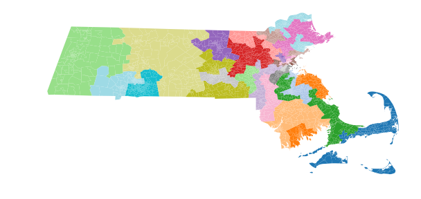
That looks like a districting plan! Woohoo! 🎉🎉🎉
Troubleshooting possible issues
If the plan looked like random noise or confetti, then we might suspect that something had gone wrong. The two places we would want to look for problems would be:
the
graph.joincall, which would go wrong if the GEOIDs did not match up correctly, orthe final
real_life_plan.plotcall, which would go wrong if the GeoDataFrame’s index did not match the node IDs of our graph in the right way.
We could inspect both issues by making sure that the records with matching IDs actually referred to the same block groups.
You also might run into problems when you go to run a Markov chain using the partition we made. If the districts are not contiguous with respect to your underlying graph, you would want to add edges (within reason) to make the graph agree with the notion of contiguity that the real-life plan uses. See What to do about islands and connectivity for a guide to handling those types of issues.